Optimization methods select the best solution from multiple options. Python’s SciPy package supports optimization; Excel’s built-in Python includes SciPy.
Single-Variable Minimization
Single-variable minimization is used directly or as a basis for multivariable optimization. SciPy uses the golden-section method and Brent’s method.
Problem: A square iron plate (side length 3m) is used to make an open-top rectangular trough by cutting equal squares from the four corners. What is the optimal size of the cut squares to maximize the trough’s volume?
Let
= side length of the cut squares. The trough’s volume is:
We maximize
over
. Since SciPy minimizes functions, we minimize
.
As shown in Figure 8-12, click cell A5, enter =PY(, and input:
def f(x):
return -(3 - 2*x)**2 * x # Minimize -f(x) to maximize f(x)
from scipy.optimize import minimize_scalar
# Bounded minimization (method='bounded'); bounds=(0, 1.5)
minimize_scalar(f, bounds=(0, 1.5), method='bounded')
Press Ctrl+Enter. Cell A5 outputs the solution (Figure 8-12):
success: True: Algorithm converged.
fun: -1.999...: Maximum volume =
(remove the negative sign).
x: 0.5: Optimal cut square side length = 0.5m.
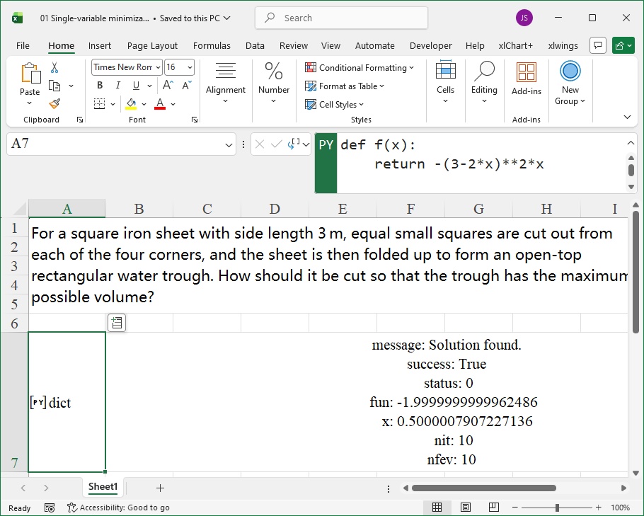
Figure 8-12 Single-Variable Minimization
Linear Programming
Linear programming (LP) requires linear objective functions and constraints. It is widely used in military, economics, industry, agriculture, education, business, and social sciences.
Problem: A factory produces two products (A and B). Producing 1 ton of A requires 3 tons of resource A and 4 m³ of resource B. Producing 1 ton of B requires 2 tons of resource A, 6 m³ of resource B, and 7 units of resource C. The economic values of A and B are 70,000 yuan/ton and 50,000 yuan/ton, respectively. Resource limits: 90 tons (A), 200 m³ (B), 210 units (C). Maximize total economic value.
Let
= tons of A,
= tons of B. The LP model is:
Since SciPy minimizes, convert to
.
As shown in Figure 8-13, click cell A8, enter =PY(, and input:
from scipy.optimize import linprog
c = [-7, -5] # Coefficients of the minimized objective function
A = [[3, 2], [4, 6], [0, 7]] # Coefficient matrix of constraints
b = [90, 200, 210] # Right-hand side of constraints
x1_bounds = (0, None) # Bounds for x₁ (≥0)
x2_bounds = (0, None) # Bounds for x₂ (≥0)
linprog(c, A_ub=A, b_ub=b, bounds=[x1_bounds, x2_bounds])
Press Ctrl+Enter. Cell A8 outputs the solution (Figure 8-13):
success: True: Algorithm converged.
x: [14.0, 24.0]: Produce 14 tons of A and 24 tons of B.
fun: -218.0: Maximum economic value = 218,000 yuan.
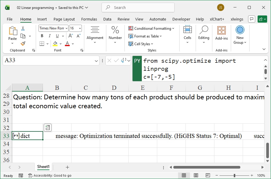
Figure 8-13 Linear Programming
This chapter covers scientific computing with Excel’s built-in Python, including calculus (Sympy), linear algebra (NumPy/SciPy), and optimization (SciPy).